
This post focuses on the accurate measurement of the number of cycles needed to execute a particular CUDA device code snippet. We will use the clock() function for the measurement and focus on adjusting the compiled device code using an assembler to get the accurate results.
Methodology
We measure the latency using the CUDA’s clock() function. This returns a counter value that is incremented in every cycle during the operation of the SM (simultaneous multiprocessor). Querying the counter at two points in the kernel code therefore can be used to compute the number of cycles elapsed while the SM executed the code placed between them. There are two major limitations of this:
- First, the counters have different starting values for different SMs, so we cannot measure inter-block execution time (if two blocks scheduled to different SMs).
- Second, the compiler can reorder instructions, so we do not exactly know the exact set of source code lines we measure. Furthermore, some instructions like shared/global memory loads have variable latency: even if the load instruction is correctly placed between two
clock()queries, the loads might not finished when the secondclock()is executed so we only measure the time needed to issue the instruction not to complete it.
The first issue cannot be reliably solved. We focus on the second. We will use an unofficial CUDA assembler combined with the official CUDA compiler to adjust the generated device code. Using this method, we can move the clock() instructions to the right place and we can explicitly set barriers to wait for variable latency instructions to be finished, thus we can measure the true latency even if variable latency ops are involved. We will use the CuAssembler in this post.
Compilation process, adjusting the device code
CUDA code is compiled in two major steps: when we call nvcc, it takes the CUDA C++ host + device code (e.g. my_kernel.cu) from which the device code is extracted and first compiled to PTX e.g. my_kernel.ptx. PTX is an architecture independent format that is further optimized and compiled to device code (SASS believed to mean shader assembly) for the specific GPU architecture with Nvidia’s proprietary compiler (ptxas). The resulting code will be in the my_kernel.sm_${sm_version}.cubin generated during the build process. The .cubin file stores the actual SASS code the GPU executes. It will be embedded into the final executable in the last steps of the compilation process by nvcc. The driver then extracts this code from the final executable at program startup. The .cubin file can be disassembled to human-readable format using CuAssembler and it can be re-assembled to .cubin after we modified the assembly source. The nvcc can be asked to use the updated .cubin code when producing the final executable. The steps we need to do are the following:
- Develop the actual source code, add the
clock()calls. - Full CUDA compilation with nvcc: this results in the executable and the
.cubin. - Disassemble the
.cubinwith CuAssembler, so we get the.cuasmfile. - Edit the
.cuasm, inject new code, configure barriers, move theclock()instruction to the right place. - Compile the
.cuasm, overwrite the first.cubin. - Ask
nvccto use the updated.cubinto compile the binary. The updated binary will have the right placement of theclock()instruction, so we can start microbenchmarking the code.
I developed a simple wrapper (cuasmw) in Python that simplifies the whole process and I also added a Jupyter notebook, so you can experiment on remote devices as well. It simplifies the process to two commands supported by cuasmw:
codec: compiles the code, disassembles to.cuasm, and executes the code, prints thread-level start-stop times to stdout.ass: once you updated the assembly code, compiles it, and updates the binary and executes it, so you instantly see the thread-level start-stop times.
I suggest to use the Jupyter notebook (visualize.ipynb) I provided as it can execute both commands and render the warp timeline graph.
Example: measuring shared memory write then read latency
Shared memory is on the chip so it is believed that its latency is only somewhat higher than the register access (that is 1-3 cycles), so we would expect it, say, 5 cycles. Let’s verify this common belief by actually measuring the elapsed cycles! One note: shared memory load (LDS) is a variable latency instruction. This means that the GPU executes subsequent independent ops before the memory is actually loaded into the LDS‘ destination register. If an upcoming instruction depends on the destination register of LDS, then, the programmer should explicitly wait on the barrier set by the LDS instruction. This causes the GPU to wait until the barrier is cleared by the memory controller preventing RAW (read after write) hazard. We will see this kind of technique first with the global memory load (LDG) instruction: the address operand of the shared memory write instruction is read from the global memory, so the compiler generates an LDG instruction that sets a wait barrier and the STS instruction waits on it, so the LDG must finish reading the data to the register before the STS is issued.
I provided a simple example code in shmem/shmem.cu that tries to measure the latency of shared memory ops: we save 4 bytes to a shared memory address, then load from the same address (sts_addr and lds_addr are the same). I also added a __synchthreads() between the shared memory load so we can make sure that the data is actually committed into the shared memory before it is executed.
template<uint N_THREADS>
__global__ void shmem_test(float* in, float* out, uint32_t* ptr, long long int* metrics){
    long long int start_a;
    long long int end_a;

    __shared__ float sh[N_THREADS];

    const uint sts_addr = ptr[threadIdx.x*2+0];
    const uint lds_addr = ptr[threadIdx.x*2+1];

    start_a = clock();
    float store_val = 42.0;
    sh[sts_addr] = store_val;
    __syncthreads();
    float load_val = sh[lds_addr];
    end_a = clock();

    out[threadIdx.x] = load_val;

    metrics[threadIdx.x*4 + 0] = start_a;
    metrics[threadIdx.x*4 + 1] = end_a;
}
We will use the visualize.ipynb to render the result. The command line interface cuasmw can be also used, but the thread statistics should be grabbed from the stdout for visualization.
When using the notebook, we need to update the main() function in the notebook:
# The same as ./cuasmw codec shmem/shmem
out = build('codec', 'shmem/shmem')
We need to see a similar warp-level statistics in the notebook:
   t | event | warp(s)
-----+-------+--------
   0 | START | [0 ]
   2 | START | [1 ]
   4 | START | [2 ]
   6 | START | [3 ]
 384 | STOP  | [0(Δt=384) 1(Δt=382) 2(Δt=380) 3(Δt=378) ]
Warp-level timelines (we use 128 threads and one single block so we will have 4 warps):
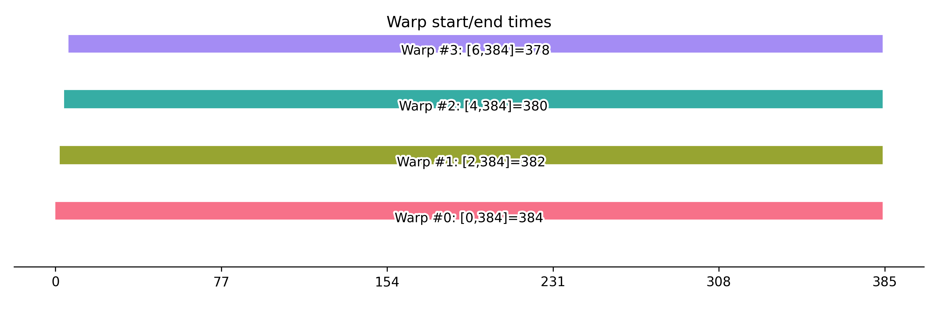
378-384 cycles for a shared memory write and then load probably is too high, so the generated device code might included global memory loads as well for example. We need to verify this by investigating the disassembled SASS code by manually reviewing the disassembled code: shmem/build-shmem/shmem.sm_75.cuasm (I use a Turing GPU, so for me the ${SM_VERSION} is 75):
$ cat shmem/build-shmem/shmem.sm_75.cuasm
...
.text._Z10shmem_testILj128EEvPfS0_PjPx:
 [B------:R-:W-:-:S02]         /*0000*/                   MOV R1, c[0x0][0x28] ;
 [B------:R-:W0:-:S01]         /*0010*/                   S2R R5, SR_TID.X ;
 [B------:R-:W-:-:S02]         /*0020*/                   MOV R10, 0x4 ;
 [B0-----:R-:W-:Y:S05]         /*0030*/                   SHF.L.U32 R2, R5, 0x1, RZ ;
 [B------:R-:W-:Y:S08]         /*0040*/                   IMAD.WIDE.U32 R2, R2, R10, c[0x0][0x170] ;
 [B------:R0:W5:-:S04]         /*0050*/                   LDG.E.SYS R0, [R2] ;
 [B------:R0:W5:-:S02]         /*0060*/                   LDG.E.SYS R4, [R2+0x4] ;
 [B------:R-:W-:-:S02]         /*0070*/                   CS2R R6, SR_CLOCKLO ;
 [B0-----:R-:W-:Y:S08]         /*0080*/                   MOV R3, 0x42280000 ;
 [B-----5:R-:W-:-:S04]         /*0090*/                   STS [R0.X4], R3 ;
 [B------:R-:W-:-:S05]         /*00a0*/                   BAR.SYNC 0x0 ;
 [B------:R0:W1:-:S02]         /*00b0*/                   LDS.U R11, [R4.X4] ;
 [B------:R-:W-:-:S02]         /*00c0*/                   CS2R R8, SR_CLOCKLO ;
 [B0-----:R-:W-:-:S01]         /*00d0*/                   SHF.L.U32 R4, R5.reuse, 0x2, RZ ;
 [B------:R-:W-:-:S01]         /*00e0*/                   IMAD.WIDE.U32 R2, R5, R10, c[0x0][0x168] ;
 [B------:R-:W-:Y:S05]         /*00f0*/                   MOV R13, 0x8 ;
 [B------:R-:W-:-:S02]         /*0100*/                   IMAD.WIDE.U32 R4, R4, R13, c[0x0][0x178] ;
 [B-1----:R-:W-:-:S06]         /*0110*/                   STG.E.SYS [R2], R11 ;
 [B------:R-:W-:-:S04]         /*0120*/                   STG.E.64.SYS [R4], R6 ;
 [B------:R-:W-:-:S01]         /*0130*/                   STG.E.64.SYS [R4+0x8], R8 ;
 [B------:R-:W-:-:S05]         /*0140*/                   EXIT ;
.L_x_0:
 [B------:R-:W-:Y:S00]         /*0150*/                   BRA `(.L_x_0);
 [B------:R-:W-:Y:S00]         /*0160*/                   NOP;
 [B------:R-:W-:Y:S00]         /*0170*/                   NOP;
.L_x_1:
...
The time measurement starts with CS2R R6, SR_CLOCKLO ; and it stops in CS2R R8, SR_CLOCKLO ; (the instruction CS2R copies the content of the special register SR_CLOCKLO to R6 at the start of the measurement then R8 at the end). We can see that the problem is with the instruction between them:
[B-----5:R-:W-:-:S04] /*0090*/ STS [R0.X4], R3 ;
waits on the 5th barrier to be cleared and it is included in the measurement (see the documentation of CuAssember or MaxAs for a detailed description of the barriers). This write barrier is set by the previous LDG (global memory load) instruction because the shared (memory store depends on it), so it is only cleared when the data is “arrived” from the global memory to the registers. Reading from the DDR ram can have multiple hundreds of cycles latency depending on many factors. We need to adjust the code to wait to this barrier before the time measurements starts, so we update shmem.sm_75.cuasm. There are other problems as well, so we adjust the following:
- Wait for the LDS and STS operands to be ready before the time measurement starts.
- Move the all instructions but LDS, STS and the memory barrier to precede the timing.
- Wait for the LDS instruction to be finished before the time measurement ends.
The updated code around the time measurement (instructions 50 to c0):
...
[B------:R0:W5:-:S04] /*0050*/ LDG.E.SYS R0, [R2] ;
[B------:R0:W5:-:S02] /*0060*/ LDG.E.SYS R4, [R2+0x4] ;
[B0----5:R-:W-:Y:S08] /*0080*/ MOV R3, 0x42280000 ;
[B------:R-:W-:-:S02] /*0070*/ CS2R R6, SR_CLOCKLO ;
[B------:R-:W-:-:S04] /*0090*/ STS [R0.X4], R3 ;
[B------:R-:W-:-:S05] /*00a0*/ BAR.SYNC 0x0 ;
[B------:R0:W1:-:S02] /*00b0*/ LDS.U R11, [R4.X4] ;
[B-1----:R-:W-:-:S02] /*00c0*/ CS2R R8, SR_CLOCKLO ;...
The updated code waits for the global memory load to be completed before we query the starting cycle number, moves the MOV instruction out of the time measurement code, and the second CS2R waits for the write barrier set by the LDS instruction, so we only execute it, after the shared memory load is completed. Note that the LDS instruction also sets a read barrier but its only purpose is to preventing overwriting the LDS source operand register that is cleared before the write barrier.
The updated code is assembled with:
# The same as ./cuasmw ass shmem/shmem
out = build('ass', 'shmem/shmem')
Now we the warp statistics is the following:
   t | event | warp(s)
-----+-------+--------
   0 | START | [0 ]
   3 | START | [1 ]
   4 | START | [2 ]
   7 | START | [3 ]
  58 | STOP  | [0(Δt=58) ]
  59 | STOP  | [1(Δt=56) ]
  61 | STOP  | [2(Δt=57) ]
  63 | STOP  | [3(Δt=56) ]
So we can execute the combined shared memory write and load in 56 to 58 cycles depending on the warp identifier, meaning that the shared memory access latency is roughly 22 to 23 cycles (we need to subtract the fixed latencies of issuing the ops.
References
https://github.com/NervanaSystems/maxas/wiki/Control-Codes
https://github.com/cloudcores/CuAssembler/blob/master/UserGuide.md
Leave a Reply